2.1 A few notational remarks

Consider the vector \(X_i = (X_1 , X_2, \dots, X_{100})\) which contains the results from a fair coinflip. Using the rbinom function we simulate n = 100 cointosses and obtain a vector of results \(x_i = (x_1, x_2, \dots, x_{100})\) :

X <- rbinom(n = 100, size = 1, prob = 0.5)

print(X)

##   [1] 0 1 0 1 1 1 0 0 0 0 0 0 0 0 1 0 1 1 1 0 0 0 0 1 1 0 1 1 0 1 1 0 1 0 0
##  [36] 0 0 1 0 1 0 1 1 0 0 1 1 0 0 0 1 1 0 0 1 0 1 0 0 0 1 0 0 1 1 0 1 1 1 1
##  [71] 1 1 1 1 0 1 1 0 1 0 0 1 0 1 0 0 1 0 0 1 1 1 0 0 0 1 0 1 0 1

If we would additionally conduct another experiment where we count two successive coin tosses (size = 2), we would obtain a second random variable, which we would denote by \(Y_i\) and \(y_i\) respectively.

Notation:

• Use capital letters such as \(O\) or \(P\) to denote a random variable
• Use small letters such as \(m\) or \(n\) to denote particual outcomes of \(M\) and \(N\)
• Use subscripts (e.g. \(a_i\)) to distinct different outcomes of the random variable \(A_i\)

2.2 Discrete random variables

Discrete random variables are variables which can only take a countable number of values. For our cointoss example, \(X\) is a random variable with \(j = 2\) outcomes, \(\{0, 1\}\) (no head, head). Then the probability of each outcome is:

\[p_j = P(X = x_j), \; j = 1, 2 \qquad \text{with } p_1 + p_2 = 1\]

Random variables which can only take on two values are called Bernoulli random variables

Example:drawing a card and predicting its symbol

• Denote the random variable for the card draw by \(C\)
• We have \(j = 4\) possible outcomes for \(C\), \(\{hearts, spades, clubs, diamonds\}\)
• The probabilities are denoted as: \(p_j = P(C = c_j), \; j= 1, 2, \dots , 4\)
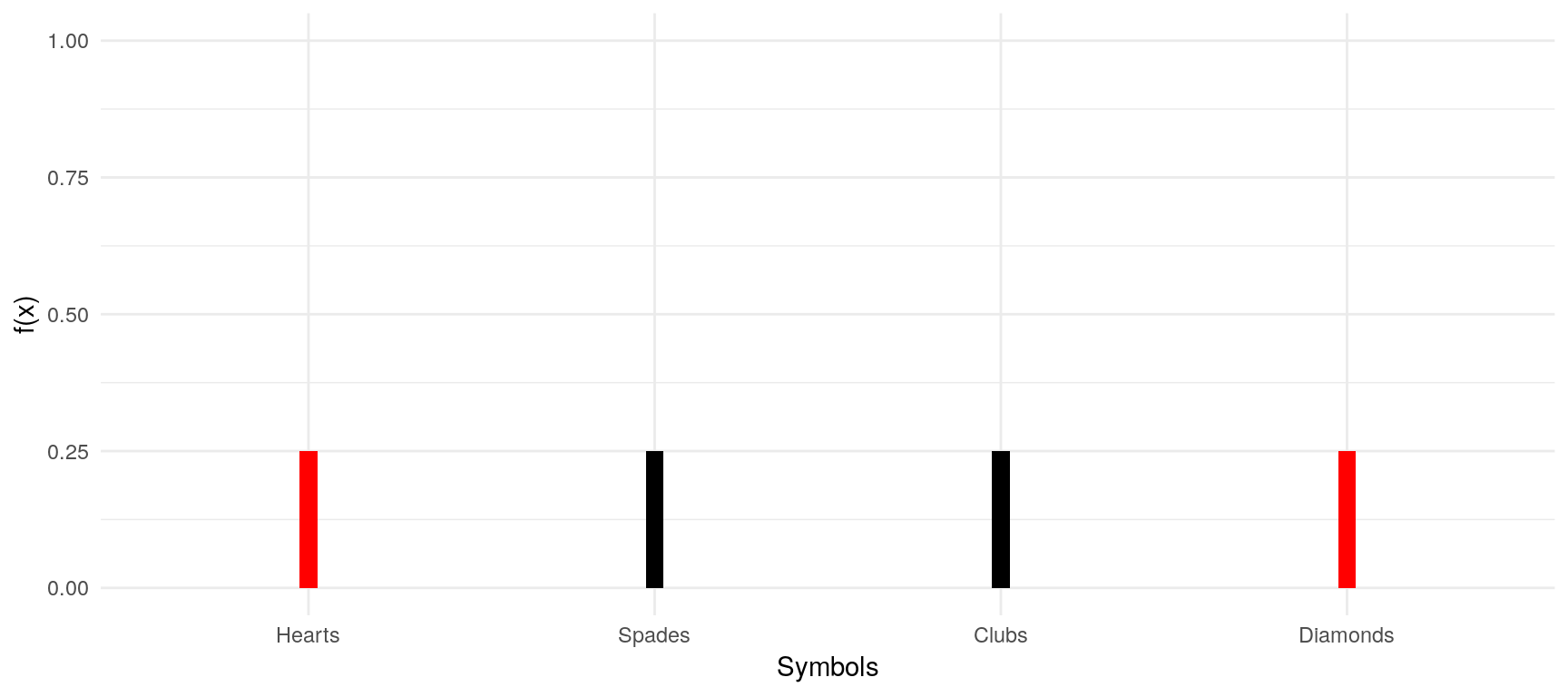
• Since we know that each symbol is represented equally in the deck, \(p_j = 0.25\) for all \(j\).
• The probability to draw a joker is \(0\) since the sample space only includes the four symbols.
• Likewise, the probability to draw any of the four symbol is \(1\) (\(100%\)).

2.3 Continuous random variables

We call a random variable continuous if it takes on any real value with a probability of \(0%\). This is because the variable could essentially take on an infinity of values and \(100%\) divided by infinity is (not possible) approaching \(0%\). Continuous random variables are seldom observed in everyday life, but one pseudo-example is the height of a person. Usually a person’s height ranges somewhere between \(45cm\) and \(272cm\). It is true that it is unlikely that someone’s height would take on a negative value or one that is generally outside the above-mentioned range. However, within the range, there is still an infinity of exact values that a person’s height can take on (consider my height: \(182,6732467cm\), still taller than my neighbour, who measures \(182,6732466cm\)).

3.1 Discrete random variables

For discrete random variables, the probability density function (pdf), or rather, the probability mass function (pmf) summarises the information concerning the possible outcomes of a discrete random variable \(X\) and its corresponding probabilities. It is defined as: \[f_X(x) = P(X=x)\] For our card symbol example, a pmf would look like this:

library(ggplot2)

p <- rep(0.25,4)
symbols <- factor(c(0,1,2,3), labels=c("Hearts","Spades",
                                         "Clubs", "Diamonds"))
df = data.frame(p, symbols)
ggplot(df, aes(symbols,p, fill=symbols)) + 
  geom_bar(stat="identity",width = 0.05) +
  scale_y_continuous(limits=c(0,1)) + labs(y="f(x)", x="Symbols") +
  scale_fill_manual("legend",
                    values = c("Hearts" = "red", "Spades" = "black",
                               "Clubs" = "black", "Diamonds" = "red")) + 
  guides(fill=F) + theme_minimal()

With this pmf, we can now simply calculate the probability of any event involving that variable. For instance, we could ask ourselves: “What is the probability that the symbol of the card that I will draw is either Hearts or Clubs?”. The pmf tells us: \[\begin{aligned}&P(X=\text{Hearts or } X=\text{Clubs})\\&=P(X=\text{Hearts}) + P(X=\text{Clubs})\\&=0.25 + 0.25 = 0.5\end{aligned}\]
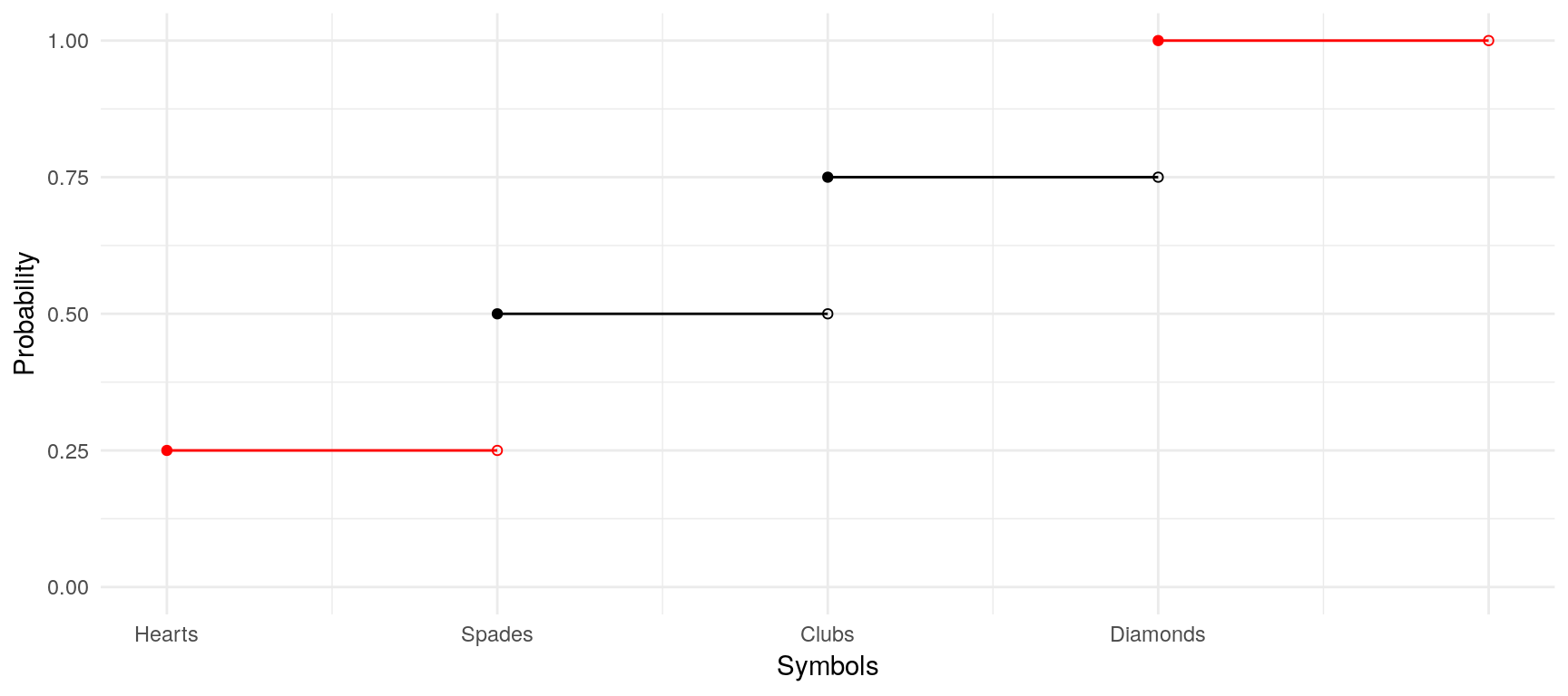
We could also answer that question with the help of the cumulative density function (cdf). As the name already suggests, the cdf cumulates the probabilities of the single possible outcomes and is defined as \[F(x) = \sum_{X\leq x}f_X(x)=P(X\leq x)\] Our current example with the cards does not really suit the benefits of a cdf, as we could indeed read from the function the probability of drawing either a Hearts card or a Spades card, but we are unable to read from it the probability of drawing either a Diamonds card or a Hearts card:

df$xend <- c(df$symbols[2:nrow(df)], 5)
df$yend <- cumsum(df$p)
ggplot(df, aes(as.numeric(symbols), cumsum(p), xend=xend, yend=yend, color=symbols)) +
      #geom_vline(aes(xintercept=as.numeric(symbols)), linetype=2, color="grey") +
      geom_point() +
      geom_point(aes(x=xend, y=cumsum(p)), shape=1) + 
      geom_segment() +
      scale_color_manual("legend",
                    values = c("Hearts" = "red", "Spades" = "black",
                               "Clubs" = "black", "Diamonds" = "red")) +
      scale_x_continuous(breaks = 1:5, 
                         labels = c("Hearts", "Spades",
                                    "Clubs", "Diamonds", "")) +
      scale_y_continuous(breaks = seq(0,1,0.25), limits = c(0,1)) +
      guides(color=F) + labs(x="Symbols", y="Probability") +
      theme_minimal()

3.2 Continuous random variables

Because it makes little sense to think about the probability that a continuous random variable assumes a certain value, the pdf of continuous random variables is used to calculate events concerning a range of values. This is done by taking the integral of this range. Generally: \[F_X(x) = \int f_X(x) dx\]

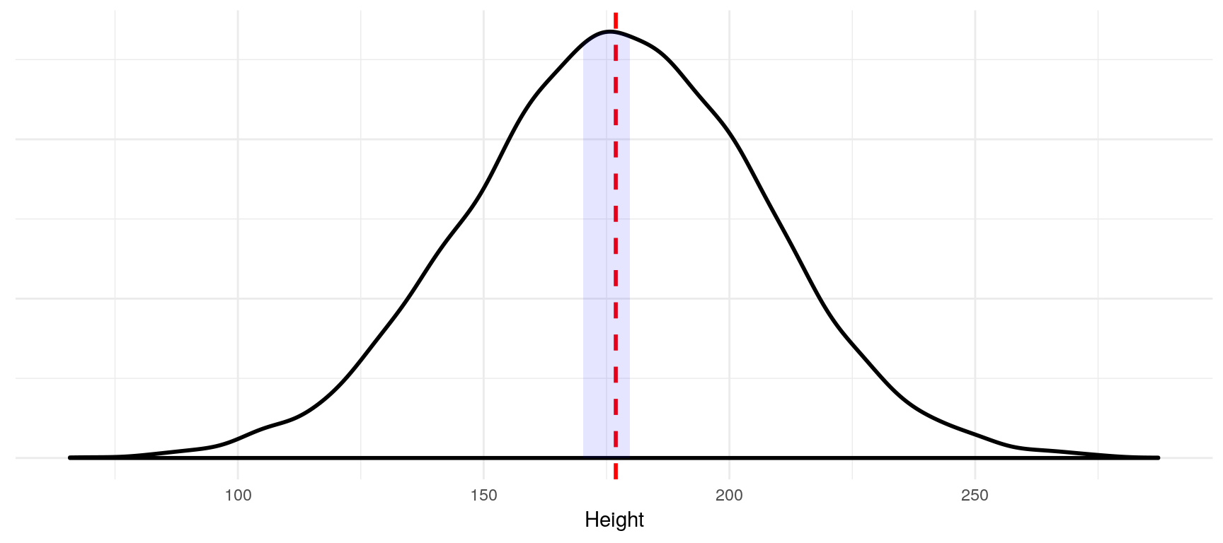
In our height example, we could be interested in the probability that a person is somewhere between \(170cm\) and \(180cm\) tall, i.e. in \(P(170\leq X \leq 180)\).

height = rnorm(10000, mean=177, sd=30)
df = data.frame(height)
dp <- ggplot(df, aes(height)) + geom_density(size=1) + 
  geom_vline(aes(xintercept=mean(height)), color="red", linetype="dashed",
                 size=1)
dpb <- ggplot_build(dp)
x1 <- min(which(dpb$data[[1]]$x >=170))
x2 <- max(which(dpb$data[[1]]$x <=180))
dp + geom_area(data=data.frame(x=dpb$data[[1]]$x[x1:x2],
                               y=dpb$data[[1]]$y[x1:x2]),
               aes(x=x, y=y), fill="blue", alpha=0.1) +
    theme_minimal() + 
    theme(axis.title.y=element_blank(),
          axis.text.y=element_blank()) + labs(x="Height")

library(sfsmisc)
dens = density(df$height)
integrate.xy(dens$x, dens$y,170,180)

## [1] 0.1327096

Thus, \(P(170\leq X \leq 180) \approx 0.13 = 13%\) (the integrate.xy function is not exact).

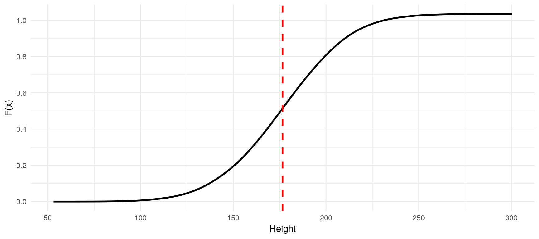
While we can calculate probabilities under the pdf for a given Range \(P(a \leq X \leq b)\), the cumulative density function always provides us with the probability of the variable to take on a value up to \(x\), that is, \(P(X \leq x)\). Its definition is: \[F_X(x)=\int_{-\infty}^xf_X(x)dx\] At all points its value is the total area under the curve of the pdf up to \(x\).

df_int = data.frame(height=dens$x, y=cumsum(dens$y)/2)
ggplot(df_int, aes(height,y)) + geom_line(size=1) + 
  geom_vline(aes(xintercept=mean(height)), color="red", linetype="dashed",
                 size=1) +
  scale_x_continuous(breaks=seq(50,300,50)) + 
  scale_y_continuous(breaks=seq(0,1,0.2)) +
  theme_minimal() + labs(x="Height", y="F(x)")

From this graph we can now easily read the probability that a person is \(150cm\) tall or smaller (ca. \(20%\)). For the requirements and attributes of probability density functions and cumulative density functions, please refer to the course slides.

4.1 Joint Distributions

The discrete case Let \(Y\) be a random variable for the throw of a die with equal chances to every side, and \(X\) a random variable for the color (blue, red) of the die. Throwing a random die would lead us to the joint probability density function of \((X,Y)\): \[f_{X,Y}(x,y) = P(X=x, Y=y)\].

It is quite easy to obtain the joint pdf of \(X\) and \(Y\) if they are independent. \(X\) and \(Y\) are independent if: \[f_{X,Y}(x,y) = f_X(x)f_Y(y)\] In other words, they are independent if the die side thrown does not depend on the color of the die. In the discrete case, it is the same as \[P(X=x, Y=y) = P(X=x)P(Y=y)\text{,}\] that is, the probability that the die is read and you throw a 6 is the product of the probability of throwing a 6 and of the die being red. Since we know these probabilities, we can calculate: \(\frac{1}{2} \times \frac{1}{6} = \frac{1}{12}\).

The continuous case By taking the integral of a joint pdf of continous variables, we can get the probability that \(X\) and \(Y\) fall in a certain interval: \[P(a \leq X \leq b, c \leq Y \leq d) = \int_a^b \int_c^df_{X,Y}(x,y)dydx\] If you have any given functions, it is quite easy (as with the normal distribution) and can be done by hand (might in some cases be easier than doing it with r). A continuous joint pdf could look like this (\(X\) = height, \(Y\) = weight; this is a bad example because obviously weight is dependent from height).

library(MASS)
library(threejs)
# Lets assume different standard deviations for height
# so that we are only looking at grown men and women
mu = c(177, 70); names(mu) = c("X", "Y")
stdevs = c(4, 5); names(stdevs) = names(mu)
cormatrix = matrix(c(1,0.9,0.9,1), ncol=2)
b = stdevs %*% t(stdevs)
varcovmat = b*cormatrix
colnames(varcovmat) = rownames(varcovmat) = names(mu)
obs = mvrnorm(n=10000, mu=mu, Sigma=varcovmat, empirical=T)
obs.kde = kde2d(obs[,1], obs[,2], n=100)

x = obs.kde$x; y = obs.kde$y; z = obs.kde$z
xx = rep(x, times=length(y))
yy = rep(y, each=length(x))
zz = z; dim(zz) = NULL
ra = ceiling(16*zz/max(zz))
col = rainbow(16, 2/3)
scatterplot3js(x=xx, y=yy, z=zz, size=0.4, color=col[ra], bg="white")

4.2 Conditional Distributions

When we are interested in the probability of a specific outcome given we observed another specific outcome, we might want to take a look at the conditional distribution of \(Y\) given \(X\), or rather, at the conditional probability density function: \[\frac{f_{Y|X}(y|x)}{f_X(x)}\] For the discrete case follows: \[f_{X|Y}(y|x) = P(Y=y|X=x)\] When \(X\) and \(Y\) are independent, it follows from \(f_{X,Y}(x,y) = f_X(x)f_Y(y)\) that \[f_{X|Y}(y|x) = f_Y(y)\text{.}\] Let us consider the die example again (\(Y\) being the colour, \(X\) the number), but lets say that if the die is blue, the chance of throwing a \(6\) is \(80%\), while the chances are distributed equally with the red die. Then: \[\begin{aligned}f_{Y|X}(6|\text{blue})&=.80\\f_{Y|X}(6|\text{red})&=\frac{1}{6}\end{aligned}\] We can also calculate \(P(X=\text{blue}, Y=6)\) if we know \(P(X=\text{blue}\). If the probability of getting the blue die is \(60%\), then \[P(X=\text{blue}, Y=6) = P(Y=6|X=\text{blue})\times P(X=\text{blue}) = .80 \times .60 = .48 = 48%\]