Linear Modelling
1 Introduction
1.1 Workflow
1.2 The lm Function
lm(formula,
   data,
   subset,
   na.action)
formula - Specification of our regression model
data - The dataset containing the variables of the regression
subset - An option to subset the data
na.action - Option that specifies how to deal with missing values
1.3 The formula Argument
- Behind the scenes, OLS-estimation is linear algebra. E.g. The linear regression parameters are derived by \(\boldsymbol{\beta} = \boldsymbol{(X'X)^{-1}X'y}\)
- In order to keep our interaction with R short and simple (and without linear algebra), R offers the formula method
We can write our models using the following syntax:
model = formula(regressand ~ regressors)Where regressand is just our dependent variable / response usually denoted by \(y\) and model is our formula of independent variables / regressors, e.g.:
happy_model = formula(happiness ~ age + income + n_children + married)We can construct formulas with the following syntax:
- Adding variables with
+
formula(y ~ a + b)- Interactions with
:
formula(y ~ a + b + a:b)- Crossing:
a * bis equivalent toa + b + a:b
formula(y ~ a + b + a:b) # and
formula(y ~ a*b) # are equivalent- Transformations with
I()
formula(y ~ a + I(a^2)) # quadratic term must be in I() to evaluate correctly
formula(y ~ log(a)) # log can stay by itself- Include all variables in your data with
.
formula(y ~ .) # is equivalent to
formula(y ~ a + b + ... + z) # for a dataset with variables from a to z- Exclude variables with
-
formula(y ~ .-a ) # is equivalent to
formula(y ~ b + c + ... + z)# for a dataset with variables from a to z
1.4 The subset Argument
- Sometimes, we want to run our model on a subset of our data
- We can specify subsets of certain variables as follows:
lm(formula,
   data,
subset = age < 30)- Connect muliple subset arguments with logical operators:
lm(formula,
   data,
   subset = age < 30 & height > 180)
Note that although this works, a best-practice is to subset your data prior to the estimation. By keeping these steps distinct, your code will be much easier for someone else to understand.
1.5 The na.action Argument
If the data contains missing values, lm automatically deletes the whole observation.
- Specify
na.action = na.failif you want an error when the data contains missing values
Again, it is a best-practice to look for missing values in your data prior to the estimation to keep your code transparent.
- You can use the
missmapfunction from theAmeliapackage to get a nice visualisation of missing values in your data
1.6 Example Call of lm with Wage Data
wage_data <- read.csv2("data/offline/wages2.csv")

head(wage_data)
## WAGE HOURS IQ SCORES EDUC EXPER TENURE AGE MARRIED BLACK SOUTH URBAN
## 1 769 40 93 35 12 11 2 31 1 0 0 1
## 2 808 50 119 41 18 11 16 37 1 0 0 1
## 3 825 40 108 46 14 11 9 33 1 0 0 1
## 4 650 40 96 32 12 13 7 32 1 0 0 1
## 5 562 40 74 27 11 14 5 34 1 0 0 1
## 6 1400 40 116 43 16 14 2 35 1 1 0 1m1 <- formula(WAGE ~ EDUC + EXPER)
model<- lm(formula = m1,
data = wage_data)1.7 Output of lm
The lm function returns a list. Relevant components of this list are:
call- the function call that generated the outputcoefficientsthe OLS coefficientsresidualsfitted.valuesThe estimates for our dpendent variable (WAGE)modelThe model matrix used for estimation
The full list of outputs can be looked up via
?lm()str(model)where model is our saved output fromlm- the
$operator andtab, e.g.model$...
Lets look up our coefficients \(\beta\), fitted values \(\hat{y}\) and OLS residuals \(\varepsilon\)
model$coefficients## (Intercept) EDUC EXPER
## -272.52786 76.21639 17.63777model$fitted.values[1:7] # first 7 fitted values## 1 2 3 4 5 6 7
## 836.0843 1293.3826 988.5170 871.3598 812.7812 1193.8631 718.9270model$residuals[1:7] # first 7 residuals## 1 2 3 4 5 6
## -67.08427 -485.38260 -163.51705 -221.35981 -250.78119 206.13686
## 7
## -118.92703We can visualise the results very simply with hist or plot:
hist(model$residuals, breaks = 30)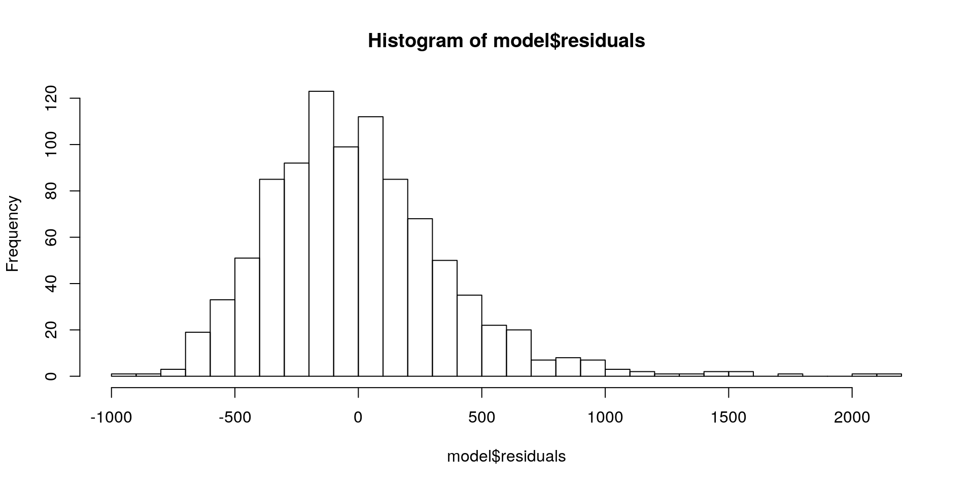
hist(model$fitted.values, breaks = 30)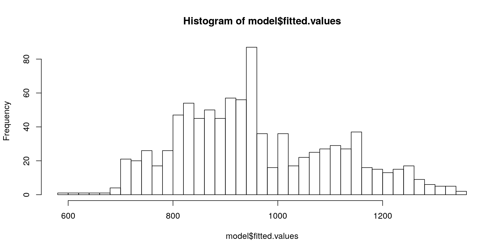
1.8 Output of lm with the summary() function
##
## Call:
## lm(formula = m1, data = wage_data)
##
## Residuals:
##     Min      1Q  Median      3Q     Max
## -924.38 -252.74  -40.88  198.16 2165.70
##
## Coefficients:
##             Estimate Std. Error t value Pr(>|t|)
## (Intercept) -272.528    107.263  -2.541   0.0112 *
## EDUC          76.216      6.297  12.104  < 2e-16 ***
## EXPER         17.638      3.162   5.578 3.18e-08 ***
## ---
## Signif. codes:  0 '***' 0.001 '**' 0.01 '*' 0.05 '.' 0.1 ' ' 1
##
## Residual standard error: 376.3 on 932 degrees of freedom
## Multiple R-squared:  0.1359, Adjusted R-squared:  0.134
## F-statistic: 73.26 on 2 and 932 DF,  p-value: < 2.2e-16
1.9 Display and Export Tables with stargazer()
stargazer::stargazer(model, type = "text", style = "asr" )##
## -------------------------------------------
## WAGE
## -------------------------------------------
## EDUC 76.216***
## EXPER 17.638***
## Constant -272.528*
## N 935
## R2 0.136
## Adjusted R2 0.134
## Residual Std. Error 376.295 (df = 932)
## F Statistic 73.260*** (df = 2; 932)
## -------------------------------------------
## *p < .05; **p < .01; ***p < .0011.9.1 Export Stargazer Output to File
stargazer::stargazer(model,
                     type = "html",
                     out = "model.html")
1.10 Compare different Models
model2 <- lm(WAGE ~ EDUC + EXPER + IQ + SCORES, data = wage_data)
stargazer::stargazer(model, model2, type = "text", style = "asr")
##
## -------------------------------------------------------------------
## WAGE
## (1) (2)
## -------------------------------------------------------------------
## EDUC 76.216*** 47.472***
## EXPER 17.638*** 13.733***
## IQ 3.795***
## SCORES 8.736***
## Constant -272.528* -536.848***
## N 935 935
## R2 0.136 0.182
## Adjusted R2 0.134 0.179
## Residual Std. Error 376.295 (df = 932) 366.466 (df = 930)
## F Statistic 73.260*** (df = 2; 932) 51.788*** (df = 4; 930)
## -------------------------------------------------------------------
## *p < .05; **p < .01; ***p < .001Specify the folder and file were your table should be saved as "path/name.type"
- Output as
.html: Open the file in your web browser and copy it into Word - Output as
.tex: Include in LaTeX
2 F-Test
2.1 Motivation of the F-Test
We can test for significance of single parameters with t-tests
- E.g. we can test if
EDUChas an influence onWAGE - We can see if the effect of
EDUCchanges when more variables are added
We can test for joint significance of a group of variables with F-tests
- E.g. are work-related variables like
TENURE,EXPERandSCORESsignificant, once we control for personal variables likeIQandEDUC
model3 <- lm(WAGE ~ IQ + EDUC, data = wage_data)
model4 <- lm(WAGE ~ IQ + EDUC + TENURE + EXPER + SCORES, data = wage_data)
2.2 Model Comparison
stargazer::stargazer(model3, model4, type = "text", style = "asr")##
## -------------------------------------------------------------------
## WAGE
## (1) (2)
## -------------------------------------------------------------------
## IQ 5.138*** 3.697***
## EDUC 42.058*** 47.270***
## TENURE 6.247*
## EXPER 11.859***
## SCORES 8.270***
## Constant -128.890 -531.039***
## N 935 935
## R2 0.134 0.188
## Adjusted R2 0.132 0.183
## Residual Std. Error 376.730 (df = 932) 365.393 (df = 929)
## F Statistic 72.015*** (df = 2; 932) 42.967*** (df = 5; 929)
## -------------------------------------------------------------------
## *p < .05; **p < .01; ***p < .0012.3 Procedure of the F-Test
- Set up the models:
- Restricted model: \(WAGE = \beta_0 + \beta_{1}IQ + \beta_{2}EDUC\)
- Unrestricted model:
\(WAGE = \beta_0 + \beta_{1}IQ + \beta_{2}EDUC + \beta_{3}TENURE + \beta_{4}EXPER + \beta_{5}SCORES\)
- State the Hypotheses that the joint effect of
TENURE,EXPERandSCORESis zero:
\[ H_0: \beta_{3} = \beta_{4} = \beta_{5} = 0 \\ H_1: H_0 \text{ is not true}\]
Since OLS minimises the \(SSR\), the \(SSR\) always increases if we drop variables. The question is, if that increase is significant.
- Calculate the test statistic:
\[ F = \frac{SSR_r - SSR_{ur}/q}{SSR_{ur} / (n-k-1)} \sim F_{q, n-k-1} \\ q = \text{number of restrictions} \\ k = \text{number of parameters}\]
If the \(H_0\) is true, our test statistic follows the \(F-Distribution\) and we can calculate p-values for our test.
2.4 F-Test in R
anova(model3, model4)## Analysis of Variance Table
##
## Model 1: WAGE ~ IQ + EDUC
## Model 2: WAGE ~ IQ + EDUC + TENURE + EXPER + SCORES
## Res.Df RSS Df Sum of Sq F Pr(>F)
## 1 932 132274591
## 2 929 124032931 3 8241660 20.576 6.495e-13 ***
## ---
## Signif. codes: 0 '***' 0.001 '**' 0.01 '*' 0.05 '.' 0.1 ' ' 1